Decoding Emotion in Vision-Language Models
Introduction
Vision-language models (VLMs) are AI models trained on text and images that create a joint representation of visual and linguistic information. VLMs are already being used for tasks such as robotics and medical image analysis. Understanding how these models encode emotion is important for developing AI technology that interacts with humans and can potentially make decisions that affect people’s well-being.
This post walks through an approach to inspect the internal workings of VLMs using sparse autoencoders (SAEs). We’ll see how to disentangle emotion-related features from VLM embeddings, visualize what the model “sees” when detecting emotions, and evaluate how well these features can predict emotion. In a follow-up post, we’ll also examine what these features reveal about bias in emotion recognition.
How VLMs Encode Emotion
VLMs encode images into high-dimensional vectors called embeddings. These embeddings exhibit a property called superposition: many features are compressed into fewer dimensions, with emotion-related information spread across multiple dimensions.
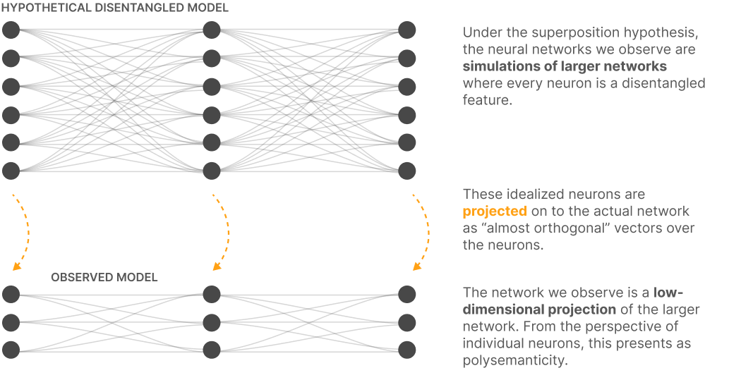
Source: Anthropic (2022)
Understanding how to disentangle these features is the key to interpretability. Using mechanistic interpretability methods, we can decompose embeddings into interpretable components.
Sparse Autoencoders
Sparse autoencoders reverse superposition by projecting representations into a higher-dimensional space. They’ve become a standard tool for vision and language interpretability.1
The three main components are:
- Projection into a higher dimensional space
- Sparsity constraint (e.g., top-k activation)
- Reconstruction loss (e.g., MSE)
Training a sparse autoencoder decomposes embeddings into monosemantic features. In essence, it unweaves the high-dimensional image representation into interpretable concepts.
class SparseAutoencoder(nn.Module):
    def __init__(self, d_in=1152, d_hidden=262_144, k=128):
        super().__init__()
        self.up_proj = nn.Linear(d_in, d_hidden, bias=False)
        self.k = k

    def forward(self, x):
        z = F.relu(self.up_proj(x))  # (B, H)
        # Keep only top-k activations per row
        vals, idxs = torch.topk(z, k=self.k, dim=-1)
        z_sparse = torch.zeros_like(z).scatter_(-1, idxs, vals)
        x_hat = F.linear(z_sparse, self.up_proj.weight.t(), bias=None)
        return x_hat

    def train_step(self, batch, optimizer):
        optimizer.zero_grad()
        x_hat = self.forward(batch)
        loss = F.mse_loss(x_hat, batch)
        loss.backward()
        optimizer.step()
        return loss.item()
Using Pre-trained SAE Features
Rather than training from scratch, we can use a pre-trained SAE trained on 210M Reddit images (available here). This gives us access to 262,144 disentangled features.
Finding Emotion-Relevant Features
We can use the EMOTIC dataset to identify the features that are related to emotion. The EMOTIC dataset contains 23k images labeled with 26 emotions. Our approach:
- Pass each EMOTIC image through the VLM to get embeddings
- Run embeddings through the SAE to get feature activations
- For each emotion, average the activation patterns across all images labeled with that emotion
- This gives us an “emotion direction” in feature space
Using these directions, we can rank any image by cosine similarity to measure alignment with each emotion. Here are the Reddit images that activate each emotion direction the most:


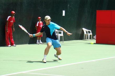


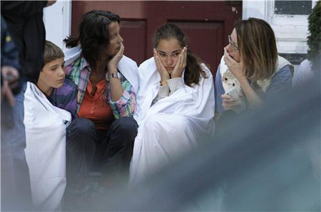
Hover over images to see heatmaps showing where emotion features activate.
Visualizing Model Attention with Heatmaps
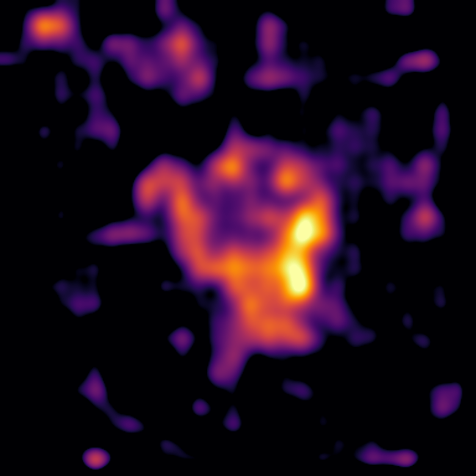
To understand where in an image the model detects emotion, we use saliency mapping, which computes gradients of the output with respect to input pixels (full code here).
- \[\begin{align*} &\text{Given: } x \in \mathbb{R}^{C \times H \times W},\quad \sigma > 0,\quad n \in \mathbb{N} \\ & G \leftarrow 0 \\ &\textbf{for } i = 1, \dots, n \textbf{ do} \\ &\quad \epsilon_i \sim \mathcal{N}(0, I) \\ &\quad \tilde{x}_i \leftarrow x + \sigma\epsilon_i\mathrm{std}(x) \\ &\quad g_i \leftarrow \frac{1}{C} \sum_{c=1}^{C} \bigl| \nabla_{\tilde{x}_i^{(c)}} f(\tilde{x}_i) \bigr| \\ &\quad G \leftarrow G + g_i \\ &\textbf{end for} \\ &S \leftarrow \frac{1}{n} G \end{align*}\]
-
G = torch.zeros_like(base[0])  # [H, W]
for _ in range(n):
    noise = torch.randn_like(base) * sigma * base.std()
    x_noised = x + noise
    x_noised.requires_grad_(True)
    y = forward(x_noised)
    g, = torch.autograd.grad(y, x_noised, create_graph=False)
    G += g.abs().mean(dim=1)
sal = G / n
We smooth the gradients by averaging over multiple noisy samples2. This reduces artifacts and produces cleaner visualizations:
| Raw Gradient | Smoothed Gradient |
|---|---|
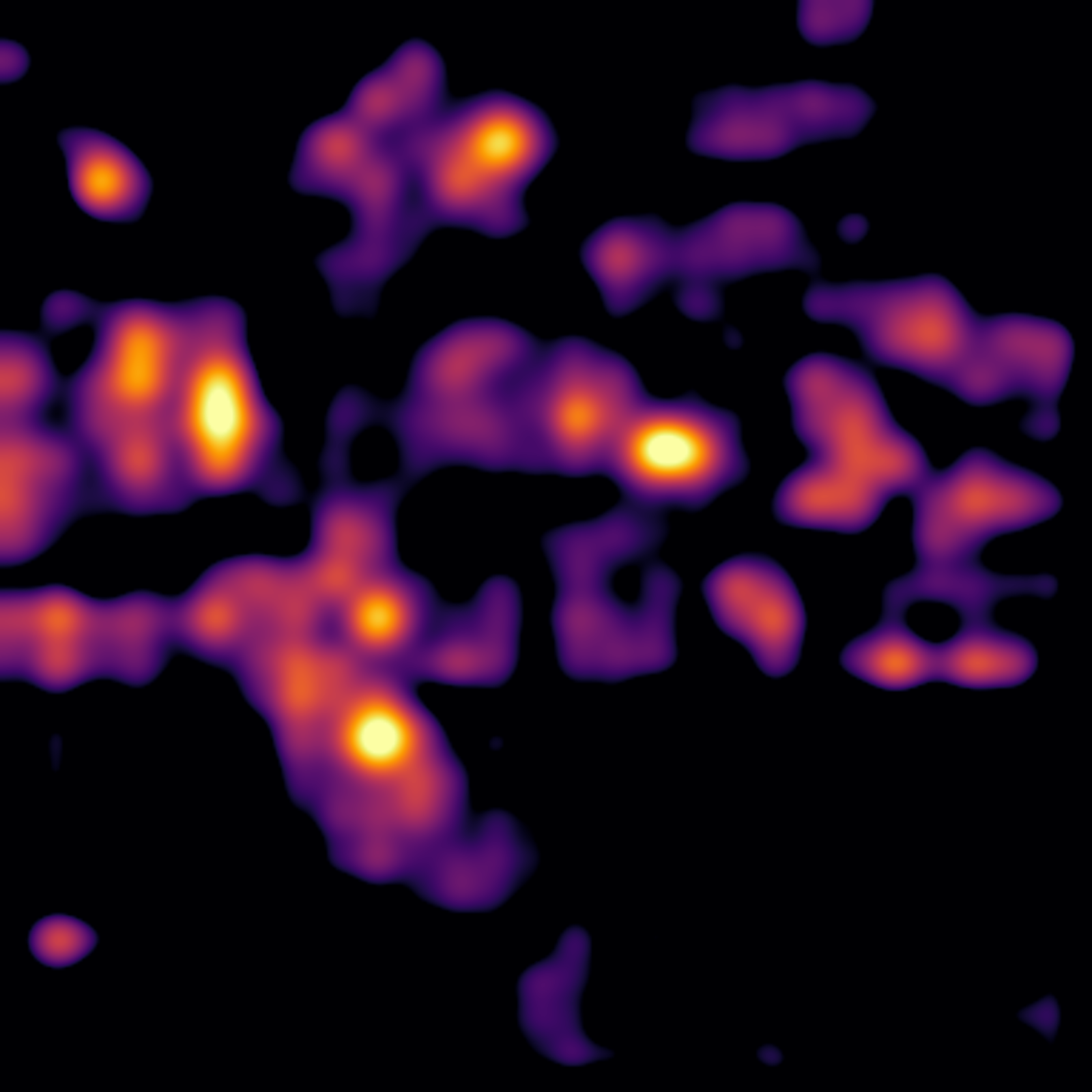 |  |
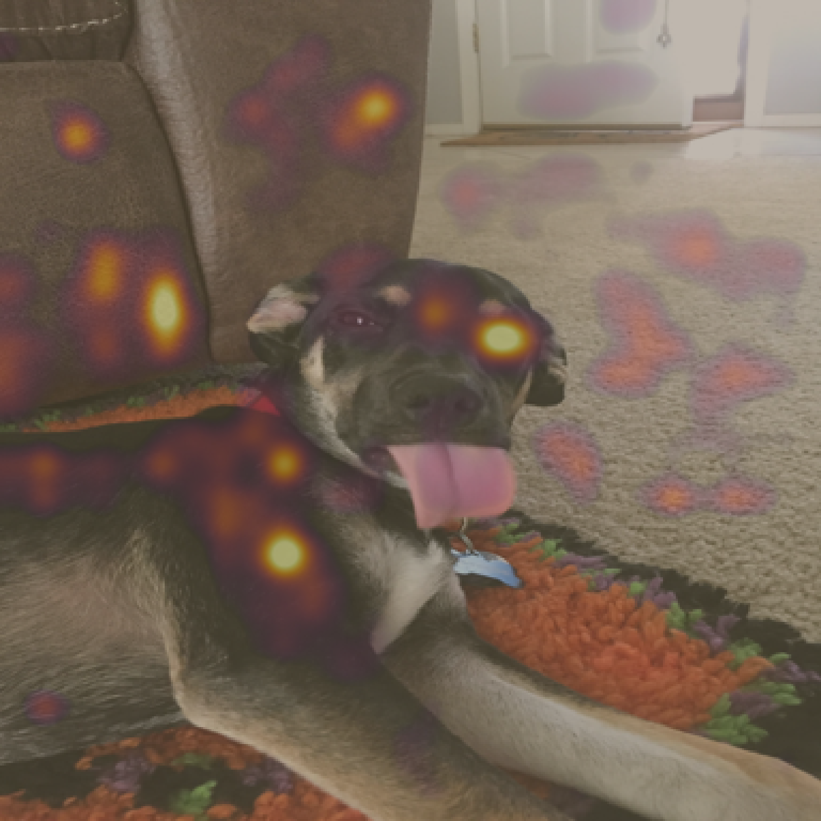 |  |
The smoothed heatmaps still contain some artifacts3, but show clear spatial localization of emotion-relevant features—impressive for a model not fine-tuned specifically for this task.
Performance Evaluation
How well can we predict emotions using just these learned directions? We evaluate on the EMOTIC test set by measuring cosine similarity between image embeddings and emotion directions and then computing average precision (AP).
Mittal et al. (2020) provide benchmark results on EMOTIC for comparison:
While not state-of-the-art, this unsupervised approach achieves reasonable performance—and crucially, gives us interpretable features we can inspect and modify.
Decomposing Emotions
I created an emotion explorer tool to help understand sparse autoencoder features. This tool displays a radial dendrogram of features, colored by the emotions they are most associated with and sized according to their activation strength. You can select a feature to query Reddit for images that most closely align with the feature:
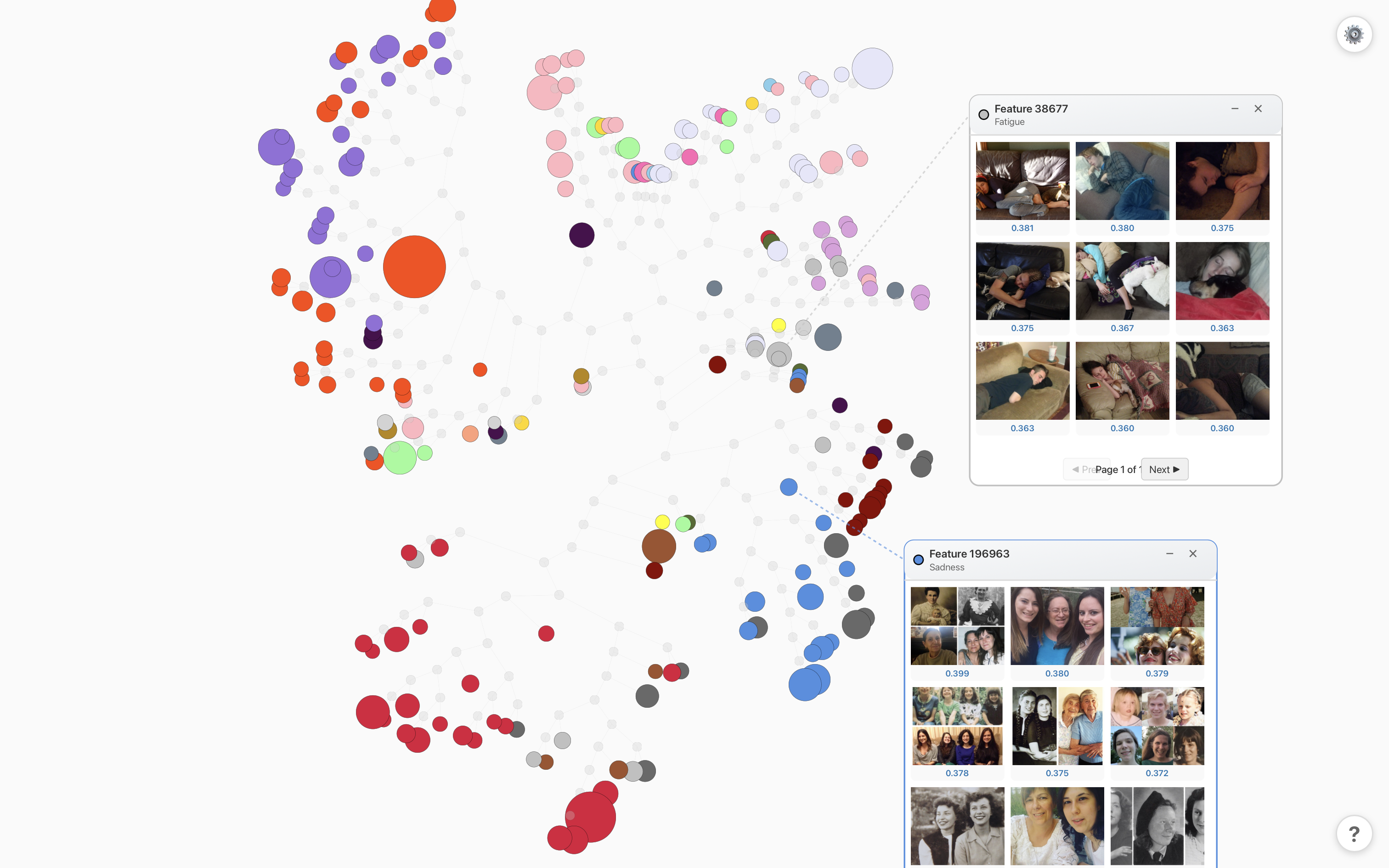
Let’s look at the top ranking features for our “Peace” direction (see the images here):
- People at the beach tanning their legs
- People passed out on couches
- Black and white photos of older people on benches
- Priests delivering sermons
- Bikes
And for “Sadness”:
- American pallbearers carrying caskets of veterans
- Ghanaian “Dancing pallbearers”, who became a popular internet meme in 2020.
- Obituary photos
- Nature documentary style photographs of African safari animals fighting.
- Pallbearers featuring other countries.
These features do not neutrally represent emotion. Instead, they reflect cultural signifiers. More specifically, they show a compound of modifiers that encode multiple layers of meaning. They are also biased toward Western culture.
Conclusion
Using sparse autoencoders, we can decompose VLM embeddings to understand how models encode emotion. This interpretability comes with practical benefits: we can visualize model attention, search images by emotional content, and identify which features contribute to predictions.
Interpretability also reveals layered meaning that is shaped by predominantly Western cultural context. In the next post, we’ll examine systematic biases in these emotion features—and explore what this means for deploying emotion recognition systems in the real world.
-
Towards Monosemanticity: Decomposing Language Models With Dictionary Learning (Anthropic (2023)). ↩
-
Smilkov et al. (2017); SmoothGrad reduces noise in gradient-based saliency maps. ↩
-
Also, attention itself is noisy. This substack post explains how ViT models sometimes stick global information in background patches. It can be mitigated by adding CLS token “registers” during training. ↩